[ Old post, left here for posterity ]

An excursion into film photography

Back in the days before Instagram in particular and digital photography in general people used little bits of plastic coated with some toxic but oh-so-magical concoction to record images. Over the years, that concoction became less toxic and eventually obsolete, but the magic never quite went away.

Disclaimer: This post was written when I had just started looking into the process of turning digitised negatives into positives. Even though I was looking for it, I had not yet found the relevant literature. As a consequence, some statements made below are inaccurate or plain wrong.

I am working on a series of posts outlining my current understanding of the process. Since life has a way of getting in the way of writing, I will make no promises about their publication date.

I am leaving this post up because I myself am often intimidated by the apparent wisdom of the authors I am reading. Let this be an example of a person who was uninformed and wrong and got a little bit smarter after a few years of digging.

These days it’s quite popular to shoot film again and I myself enjoy running a roll of Kodak’s finest through my camera from time to time.

The challenges of analog photography are quite different from what digital throws at you, but one that has vexed me in particular is the hassle of digitising film. Lab scans are either expensive and/or low quality, so they are out for me. If, however, you have ever tried to digitise colour negative film yourself, you will have found that it is all but trivial to get the colours to look right. There is a plethora of articles on subject, some of them excellent, however most conclude that you just have to feel your way through the colour adjustment.

I don’t accept that. There’s no way generations of photographers and highly trained chemists would have let such an unscientific approach to colour stand for decades.

N.B.: I am not claiming that the solution presented here is superior to manual adjustment by a trained eye. In fact, it probably isn’t, I have not done enough research for that yet.

This is merely the first step on the way to an accurate negative-positive conversion algorithm. For the moment it may or may not be useful to you as a way to automate parts of your current workflow and it may or may not provide higher quality results than your scanner software’s conversion algorithm.

A primer on colour negative film

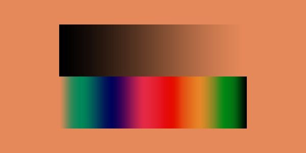
There is plenty of information out there on how colour negative film works and this article is not about that, but here’s a quick rundown for the uninitiated: the plastic base is coated with photosensitive cyan, magenta and yellow dyes (each on their own layer). Since these might have slight impurities in them, the plastic base is coloured orange to mask those imperfections. When printing in a darkroom, the photographer would dial in a combination of colour filters to remove that mask.

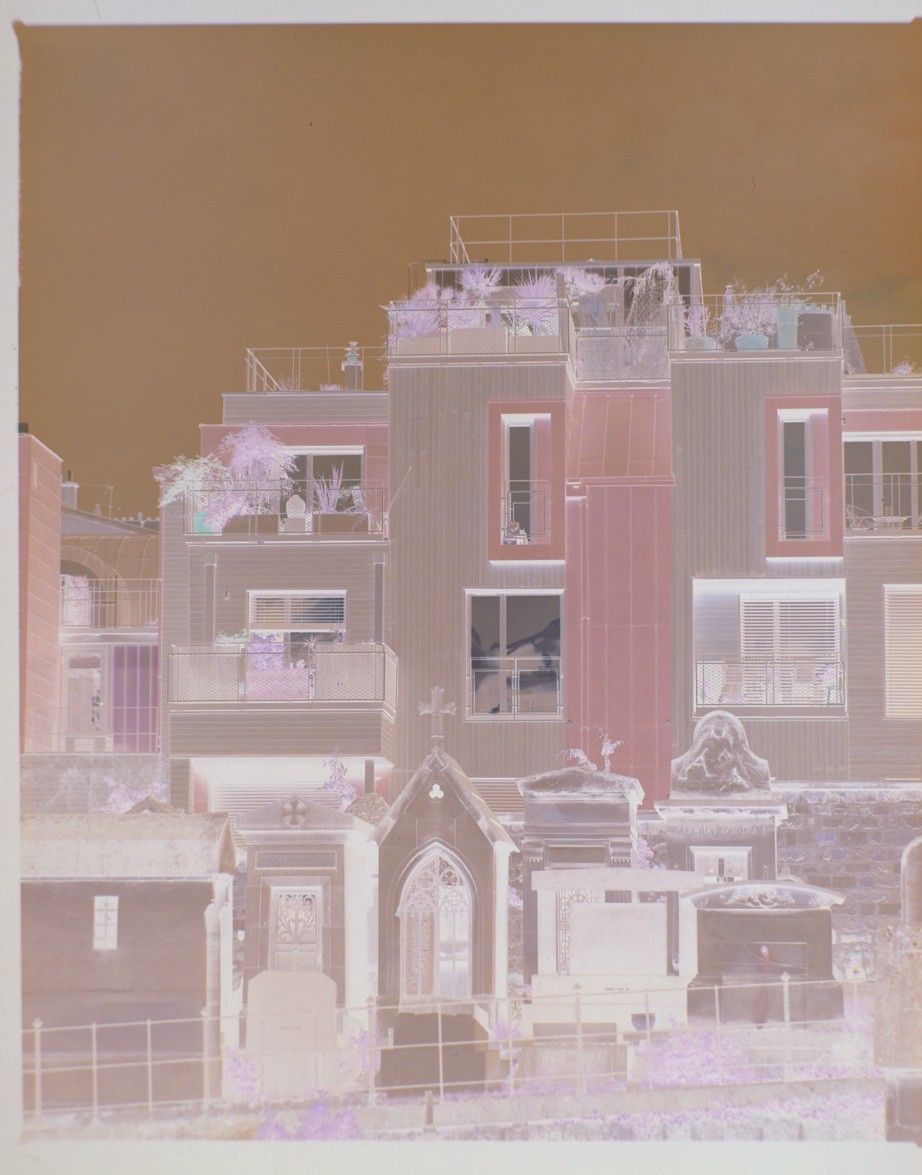
In addition to the orange base, the negative is also extremely low contrast, the idea being that the film should have more exposure latitude than strictly necessary so that a variety of extremely high contrast scenes can be reproduced naturally. In the darkroom this flat, linear curve would be transformed into a slightly steeper (read: more contrasty) S-curve by use of the appropriate paper and development process.

If you want to know more, this excellent article talks about the characteristic curve and exposure latitude of colour negative film.

Applying the darkroom playbook to digital imaging

At this stage I am going to assume you have a linear scan of your photo to work on (or, better yet, the raw data of whichever sensor you are using).

The first step is to get rid of the orange base. This is fiddly at best if you do it with the levels tool in Photoshop, but since we are programmers we can do better: no spot on the image should be a lighter colour than a patch of unexposed film. This patch will be exactly the colour of the orange base. It should be white, though.

In an ideal world we could just include a bit of the films border in our scan and run over all the pixels until we find the lightest. Unfortunately real world sensors introduce noise and since there may be light-coloured dust on the film all bets are off. To get a more reliable value, we take the average of a larger area sampling — either another image containing just the orange base (e.g. taken from the leader of the film) or the average of the lightest patch of pixels. In my implementation I opted for the former.

Having found the colour of our orange base, we can now scale all pixel values so that the base ends up being white. To maintain the largest possible precision, the image should be exposed so that the orange base is nearly white already (clipped values should be avoided at all cost, though).

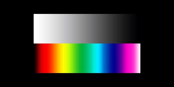
Now that our colours are simply inverted, we can convert the image to a positive by subtracting every pixel value from one. As a final touch we might want to scale the values such that the brightest channel maxes out at exactly one (meaning that pixel values will be contained in the interval ((0, 0, 0), (r_max, g_max, b_max)) such that at least one of r_max, g_max and b_max is exactly equal to one and none of them are larger than one).

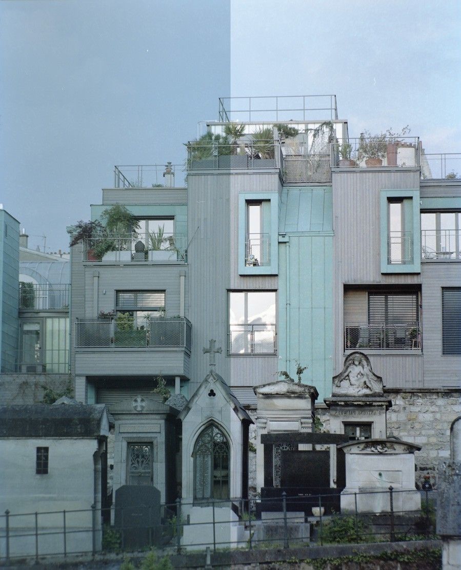
This image will still look rather flat. That’s exactly what we want, though. We can treat this as the raw file which we can use as a base for more creative adjustments.

Code

First of all: the orange mask. As discussed above, the colour of the mask might not be a hundred percent homogenous, so we use an area to average over. This is quite simply achieved by applying OpenCV’s mean function:

if args.base:
    base = cv2.imread(args.base, cv2.IMREAD_UNCHANGED)
    base = np.float32(base) / np.iinfo(base.dtype).max
    base = cv2.mean(base)

If the user doesn’t want to provide a base colour image to form our average from we can also provide a fallback function that searches for the lightest pixel in the image. As was described above this is not ideal, but since it serves only as a fallback, I consider it good enough for this experiment.

def find_base(neg, print_progress=False):
    white_sample = [0, 0]
    previous_max = 0
    
    for y in range(neg.shape[1]):
        if print_progress:
            progress = y/neg.shape[1] * 100
            if progress.is_integer():
                print(
                    ERASE_LINE+f'Searching for base: {progress} %',
                    end='\r'),
        for x in range(neg.shape[0]):
            local_max = 0
            for chan in range(neg.shape[2]):
                local_max += neg.item(x, y, chan)
            if local_max > previous_max:
                previous_max = local_max
                white_sample = [x, y]
                
    return [ neg.item(white_sample[0], white_sample[1], chan)
        for chan in range(neg.shape[2]) ]

Almost all the operations used here are traversing the entire image and thus run in O(n), that is linear, time. For large images linear time is rather slow, hence it is advisable to use the average_base procedure with a small-ish source image (I don’t have the impression that OpenCV is making use of parallelisation for these particular operations).

The find_base function runs even slower than cv2.mean or OpenCV’s mathematical operators since it is implemented entirely in Python. It could probably also be optimised a bit.

Once we know what colour the orange mask is, we can use this to white-balance the negative. Afterwards it is simply inverted. Inside the invert function I am also normalising the values to fit the range (0, 1). This is beneficial since at this point we are still working with float data. If we were to save the image as a 16 bit TIFF without scaling the range of values we might lose data that could have otherwise been preserved.

def invert(neg, base, print_progress=False):
    if print_progress:
            print(
                ERASE_LINE + 'Removing orange mask...', end='\r'),
    
    # remove orange mask
    b,g,r = cv2.split(neg)
    b = b * (1 / base[0])
    g = g * (1 / base[1])
    r = r * (1 / base[2])
    res = cv2.merge((b,g,r))
    
    if print_progress:
            print(
                ERASE_LINE + 'Inverting...', end='\r'),
    
    # invert
    res = 1 - res
    
    if print_progress:
            print(
                ERASE_LINE + 'Normalizing...', end='\r'),

    res = cv2.normalize(res, None, 0.0, 1.0, cv2.NORM_MINMAX)
    
    return res

You can find the entire program on my GitHub: https://github.com/JanHett/proto-alchemist. This implementation will probably evolve, so if you are reading this in the future, do check over there for an up-to-date implementation.

Discussing the results

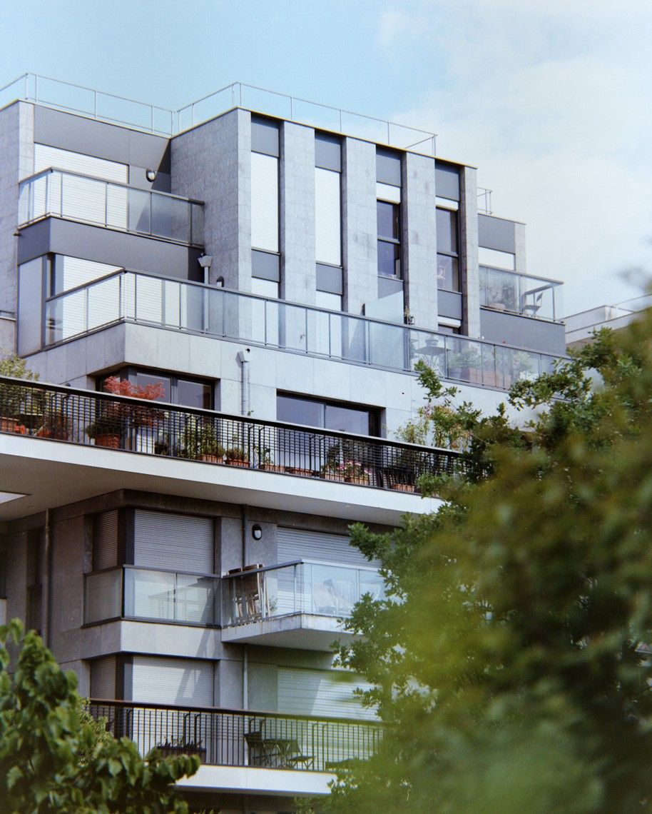
It is hard to judge the accuracy of this program objectively. The photograph shown above and the previously treated image were both digitised under less than perfect conditions: the backlight was provided by an iPad, the camera was set up on a shaky tripod and the lenses used (a Sony FE 55mm f/1.8 and a Zeiss Planar 85mm f/1.4 ZF) are entirely unsuited for reproduction photography. As noted below the images, they were also taken on expired film (which was not refrigerated for most of its life), hence even a perfect digitisation would probably exhibit strong discolouration.

That being said, I do think that the resulting positives are rather promising, though. To get comparable colours would have required much tweaking in most scanning software.

I have not yet tried the algorithm on a real world photograph of a calibration target. This would allow me to actually measure the deviation from the “correct” outcome. True to the statement made in the introduction, I do intend to do this once some of the problems of the current program are ironed out.

While the algorithm described here seems to work well enough, I have blatantly ignored a host of issues so far. Here’s just a partial list:

• Gamma
• Colour space
• Raw conversion

The problems are not even limited to the digital realm, here are a few that need to be addressed in my capture setup:

• Sensor characteristics (specifically calibration)
• Lens characteristics
• CRI, evenness and stability of the light source

Some of these points are quietly solved by OpenCV or my raw processor (Phase One’s Capture One) but the fact of it is that many loose ends remain.

Next Steps

Since my program runs multiple linear-time operations, it can get rather slow for large images. This could be sped up if we were to parallelise these operations. Additionally I would like to allow reading raw files to avoid having the additional, lossy step of raw conversion before I can run my program.

I am also experimenting with an idea for automatic dust-removal using polarised light and inpainting algorithms.

If you spot an error in my research or my code, please let me know.